Approximating Binomial with Poisson
It is usually taught in statistics classes that Binomial probabilities can be approximated by Poisson probabilities, which are generally easier to calculate. This approximation is valid “when \(n\) is large and \(np\) is small,” and rules of thumb are sometimes given.
In this post I’ll walk through a simple proof showing that the Poisson distribution is really just the Binomial with \(n\) (the number of trials) approaching infinity and \(p\) (the probability of success in each trail) approaching zero. I’ll then provide some numerical examples to investigate how good is the approximation.
Proof
The Binomial distribution describes the probability that there will be \(x\) successes in a sample of size \(n\), chosen with replacement from a population where the probability of success is \(p\).
Let \(X \sim Binomial(n, p)\), that is
\[\begin{equation} \tag{1} P(X = x) = {n\choose x} p^x (1-p)^{n-x}, \end{equation}\]
where \(x= 0, 1, \dots, n\). Define the number
\[\lambda = np\]
This is the rate of success. That’s the number of trials \(n\)—however many there are—times the chance of success \(p\) for each of those trials. If we repeat the experiment every day, we will be getting \(\lambda\) successes per day on average.
Solving for \(p\), we get:
\[ p = \frac{\lambda}{n}\] We then substitute this into (1), and take the limit as \(n\) goes to infinity
\[ \lim_{n \to \infty}P(X = x) = \lim_{n \to \infty} \frac{n!}{x!(n-x)!} \bigg( \frac{\lambda}{n} \bigg)^x \bigg( 1-\frac{\lambda}{n} \bigg)^{n-x}\]
I then collect the constants (terms that don’t depend on \(n\)) in front and split the last term into two
\[\begin{equation} \tag{2} \frac{\lambda^x}{x!} \lim_{n \to \infty} \color{blue}{\frac{n!}{(n-x)!} \bigg( \frac{1}{n} \bigg)^x} \color{red}{ \bigg( 1-\frac{\lambda}{n} \bigg)^n } \color{green}{\bigg( 1-\frac{\lambda}{n} \bigg)^{-x}} \end{equation}\]
Now let’s take the limit of this right-hand side one term at a time.
- We start with the blue term
\[\color{blue}{ \lim_{n \to \infty} \frac{n!}{(n-x)!} \bigg( \frac{1}{n} \bigg)^x }\] The numerator and denominator can be expanded as follows
\[\color{blue}{ \lim_{n \to \infty} \frac{(n)(n-1)(n-2)\dots(n-x)(n-x-1)\dots (1)}{(n-x)(n-x-1)(n-x-2)\dots (1)}\bigg( \frac{1}{n} \bigg)^x }\]
The \((n-x)(n-x-1)\dots(1)\) terms cancel from both the numerator and denominator, leaving the following
\[\color{blue}{ \lim_{n \to \infty} \frac{(n)(n-1)(n-2)(n-x+1)}{n^x} }\] This can be rewrited as
\[\color{blue}{ \lim_{n \to \infty} \frac{n}{n} \frac{(n-1)}{n} \frac{(n-2)}{n} \frac{(n-x+1)}{n} }\] This is because there were \(x\) terms in both the numerator and denominator. Clearly, every one of these \(x\) terms approaches 1 as \(n\) approaches infinity. So we know this just simplifies to one. So we’re done with the first step.
- Now we focus on the red term of (2)
\[\color{red}{ \lim_{n \to \infty} \bigg( 1-\frac{\lambda}{n} \bigg)^n }\]
Recall the definition of \(e= 2.7182\dots\) is
\[ \lim_{a \to \infty} \bigg(1 + \frac{1}{a}\bigg)^a\] Our goal here is to find a way to manipulate our expression to look more like the definition of \(e\), which we know the limit of. Let’s define a number \(a\) as
\[ a = -\frac{n}{\lambda}\]
Substituting it into our expression we get
\[ \color{red}{ \lim_{n \to \infty} \bigg( 1-\frac{\lambda}{n} \bigg)^n = \lim_{n \to \infty} \bigg( 1+\frac{1}{a} \bigg)^{-a\lambda} = e^{-\lambda} }\] So we’ve finished with the middle term.
- The third term of (2) is
\[\color{green}{ \lim_{n \to \infty} \bigg( 1-\frac{\lambda}{n} \bigg)^{-x} }\] As \(n\) approaches infinity, this term becomes \(1^{-x}\) which is equal to one. And that takes care of our last term.
Putting these together we can re-write (2) as
\[ \frac{\lambda^x}{x!} \lim_{n \to \infty} \color{blue}{ \frac{n!}{(n-x)!} \bigg( \frac{1}{n} \bigg)^x} \color{red}{ \bigg( 1-\frac{\lambda}{n} \bigg)^n} \color{green}{ \bigg( 1-\frac{\lambda}{n} \bigg)^{-x} } = \frac{\lambda^x}{x!} \color{red}{ e^{-\lambda} }\] which is the probability mass function of a Poisson random variable \(Y\), i.e
\[P(Y = y) = \frac{\lambda^y}{y!} e^{-\lambda}\]
where \(y = 0, 1, \dots\). So we have shown that the Poisson distribution is a special case of the Binomial, in which the number of trials grows to infinity and the chance of success in any trial approaches zero. And that completes the proof.
Casella and Berger (2002) provide a much shorter proof based on moment generating functions.
A natural question is how good is this approximation? It turns out it is quite good even for moderate \(p\) and \(n\) as we’ll see with a few numerical examples.
Code
A rule of thumb says for the approximation to be good:
“The sample size \(n\) should be equal to or larger than 20 and the probability of a single success, \(p\), should be smaller than or equal to 0.05. If \(n\) > 100, the approximation is excellent if \(np\) is also < 10.”
Let’s try a few scenarios. I have slightly modified the code from here.
# plots the pmfs of Binomial and Poisson
pl <- function(n, p, a, b) {

   clr <- rainbow(15)[ceiling(c(10.68978, 14.24863))]
   lambda <- n * p
   mx <- max(dbinom(a:b, n, p))

   plot(
      c(a:b, a:b),
      c(dbinom(a:b, n, p), dpois(a:b, lambda)),
      type = "n",
      main = paste("Poisson Approx. to Binomial, n=", n, ", p=", p, ", lambda=", lambda),
      ylab = "Probability",
      xlab = "x")
   points((a:b) - .15,
          dbinom(a:b, n, p),
          type = "h",
          col = clr[1],
          lwd = 10)
   points((a:b) + .15,
          dpois(a:b, lambda),
          type = "h",
          col = clr[2],
          lwd = 10)
   legend(b - 3.5, mx, legend = c("Binomial(x,n,p)", "Poisson(x,lambda)"), fill = clr, bg = "white")
}
I start with the recommendation: \(n\) = 20, \(p\) = 0.05. This gives \(\lambda= 1\). Already the approximation seems reasonable.
pl(20, 0.05, 0, 10)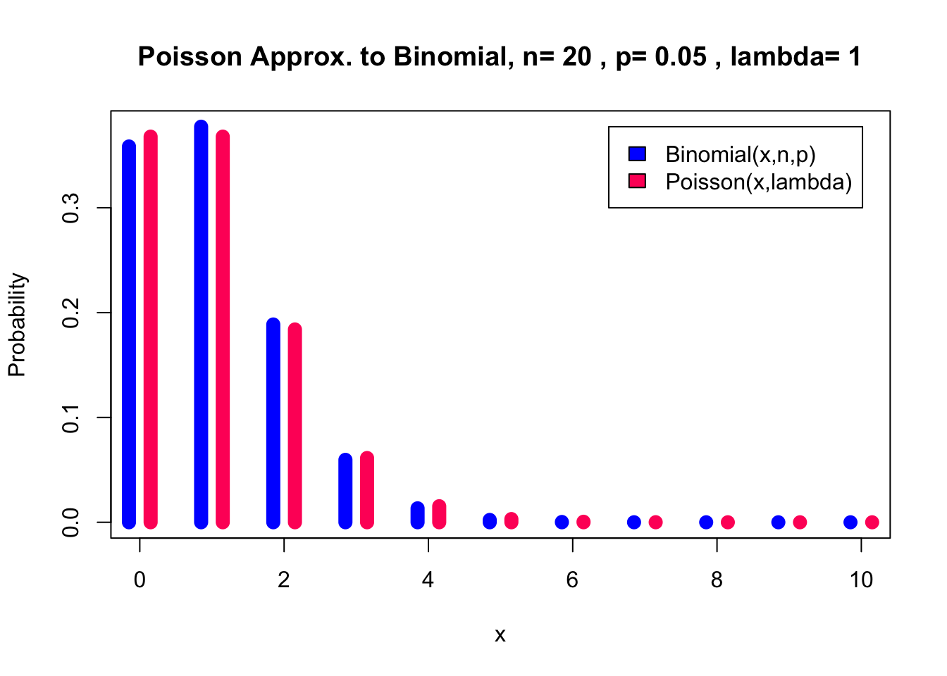
For \(n\) = 10, \(p\) = 0.3 it doesn’t seem to work very well.
pl(10, 0.3, 0, 10)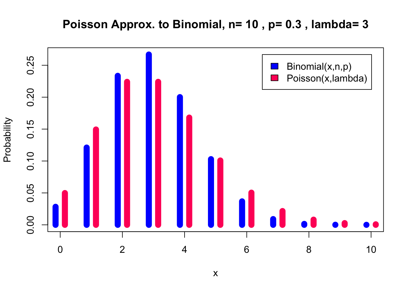
But if we increase \(n\) and decrease \(p\) in order to come home with the same \(\lambda\) value things improve.
pl(100, 0.03, 0, 10)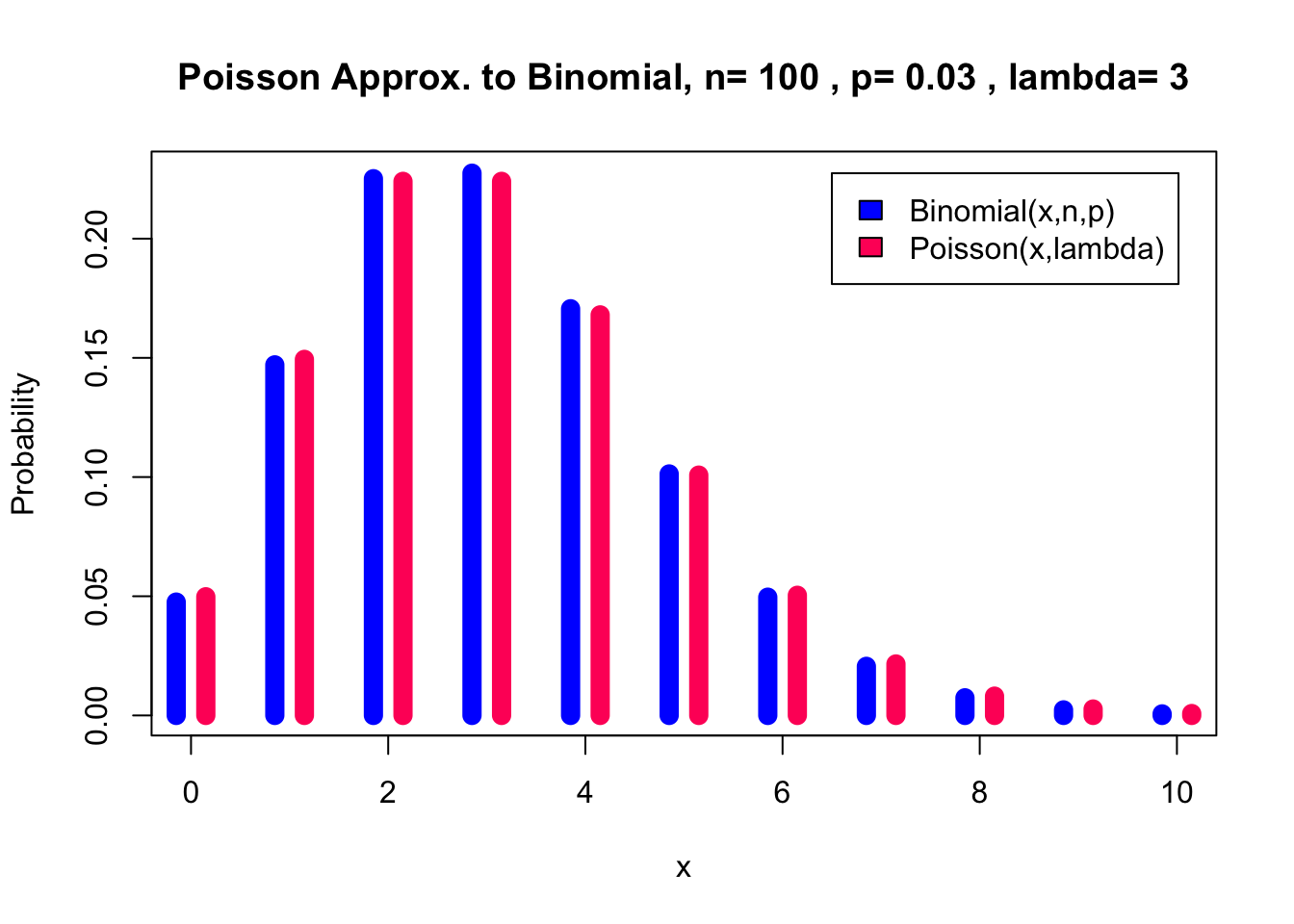 Lastly, for 1000 trials the distributions are indistinguishable.
pl(1000, 0.003, 0, 10)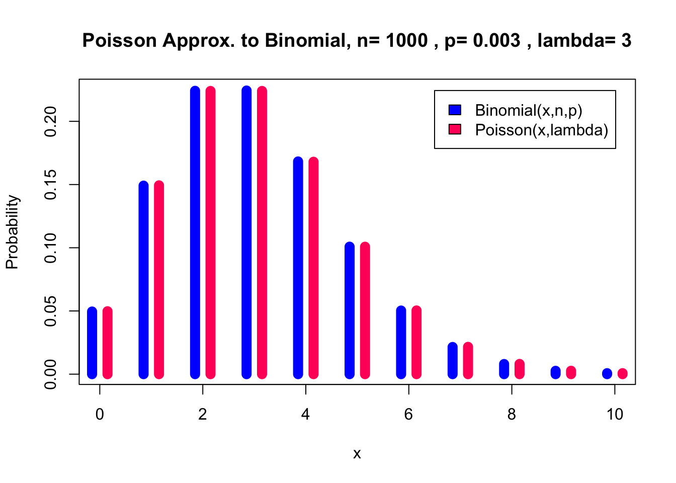
References
Casella, George, and Roger L Berger. 2002. Statistical Inference. Vol. 2. Duxbury Pacific Grove, CA.