QWERTY-nomics, how did QWERTY came to be?
QWERTY has become the dominant keyboard standard, used by billions of people every day. The basic QWERTY form was developed in 1873 and was based around four rows with eleven characters in each row.
QWERTY takes its name from the first six letter of the second line (see image).
There has been a lot of debate on the nature of QWERTY, whether the specific keyboard design was by choice or chance?
A common view is the letters QWERTY were assembled (on purpose) in one row so the salesman could impress the customers by quickly typing “typewriter” which was the name of the brand producing the hardware - “the Sholes and Glidden Type Writer”. Effectively a sales trick!
Using the six letters in QWERTY we can type the word “typewriter”.
Kay (2013) labels this view as Myth 1.
They used probability theory to investigate whether this feature of the keyboard exists “by intent or accident”. To do this, they calculated the probability the seven letters that make up “typewriter” falling on one line. This probability is 0.0002, so small, which indicates it was a design choice.
Crucially, this calculation is based on the assumption that the designer had chosen in advance to place 10 letters at the top row of the keyboard1.
Here, I’m looking how this probability changes for other values of letters at the top row.
The calculation in Kay (2013)
First, I briefly go through the calculations presented in Kay (2013). The problem is parallel to sampling without replacement from an (imaginary) urn. The designer has chosen \(K=10\) letters to be assigned at the top row of the keyboard and the rest \(R=26-10=16\) to the other rows (there are \(N=26\) letters in the alphabet).
We are interested in the probability the \(k=7\) letters needed to form the word “typewriter” finish at the top row. This probability is described by a hypergeometric distribution.
The hypergeometric distribution describes the probability of \(k=7\) “successes” in \(n=7\) draws, without replacement, from a finite population of size \(N = 26\) letters that contains exactly \(K = 10\) objects with that feature, wherein each draw is either a success or a failure. Using the usual urn-style language of “green” and “red” marbles we have:
- \(K = 10\) green marbles (i.e. 10 letters to be assigned at the top row)
- \(N = 26\) (i.e. the letters of the alphabet)
- \(R = 16\) red marbles (i.e. the rest of the letters to be assigned to the other rows)
- \(k = 7\) letters that form the word “typerwriter”
We then draw \(n = 7\) marbles without replacement. What is the probability that exactly \(k=7\) are green? This is given by
\[P(X=k) = \frac{ {K\choose{k}} {{N-k}\choose{n-k}}}{N\choose n}\]
For \(k=7, n=7, N=26, K= 10\), this probability is 0.00018 which is quite small. Hence, it indicates this was a design choice rather than by chance.
But this calculation is based on the assumption: the designer decided the number of letters for the top row to be 10 (\(K=10\)).
An updated calculation
Another approach is to change the number of letters in the top row and see how this probability changes.
Now we are interested in the probability of drawing “\(k=7\) green marbles in \(n=7\) draws for different choices of \(K\)”. The plot shows the probability of \(k=7\) for different values of \(K\). We start with \(K = 6\) which gives probability = 0, as there is no way to draw 7 green marbles when there are only 6 of them! The red dot corresponds to \(K=10\) which has been used in the paper by Kay. For \(K=19\) which corresponds to the quite extreme scenario of having 19 letters at the top row, the probability the 7 “typerwriter” letters are found there becomes 8%. Still small but appreciable.
The calculations above are based on sampling the letters in “typewriter” at any order. We can also calculate the probability of drawing “Exactly \(k=7\) green marbles in \(n=7\) draws, in the specific QWERTY order”. This corresponds to the horizontal dashed line in the plot.
Overall, adding more letters at the top row increases the probability substantially. For example, the probability increases by 9900% (!) when going from \(K=10\) to \(16\) letters. Nevertheless, in absolute terms even for \(K =19\) it is so small that we can conclude it is unlikely that these letters would appear together by chance.
For a more historical perspective and other myths on QWERTY - read this article.
library(purrr)
N <- 26
K <- seq(6, N - 7, by = 1)
prbs <- map_dbl(K, ~ dhyper(x = 7, m = .x, n = N - .x, k = 7))
df <- data.frame(K, prbs)
library(ggplot2)
library(dplyr)
# prb of exact "qwerty" word sampled
pr_exact <- (1/26)*(1/25)*(1/24)*(1/23)*(1/22)**(1/21)*(1/20)*(1/19)
ggplot(df) +
geom_point(aes(x = K, y = prbs)) +
labs(y = "Probability", x = "K") +
geom_point(data = df %>% filter(K == "10"), aes(x = K, y = prbs), col = 'red') +
geom_hline(yintercept = pr_exact, linetype = "dashed") +
scale_x_continuous(breaks = K, labels = K) +
theme_bw()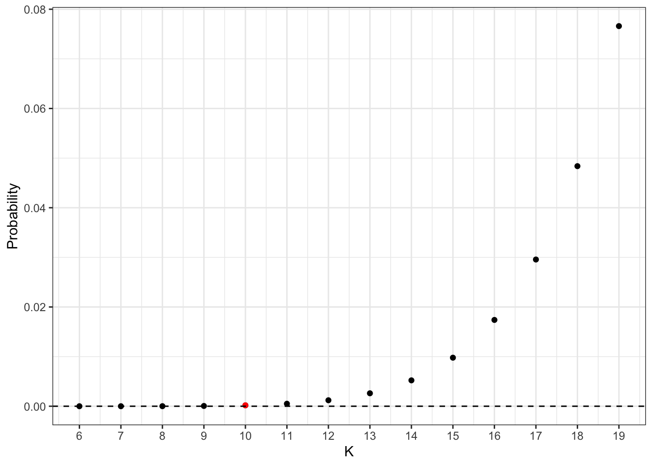
References
In fact, later versions changed this arrangement to 10 (top), 9 (middle), 7 (bottom), a more balanced ordering - this the modern QWERTY.↩︎