Recently, I came across this very interesting article published in Science about how plastic waste is associated with disease on coral reefs (J. B. Lamb et al. 2018). The main conclusions are

1. contact with plastic increases the probability of disease,
   
2. the morphological structure of the reefs is associated with the probability of being in contact with plastic with more complex ones being more likely to be affected by plastic,
   
3. the plastic levels correspond to estimates of mismanaged plastic waste into the ocean.

Overall, this study provides evidence how plastic waste negatively affects coral reefs, making them more susceptible to diseases. The authors made available both the datasets they used and the code (both can be downloaded from J. Lamb et al. 2018 - an excellent example of reproducible research). The methods section is straightforward to follow (see Supplementary Materials). My comment is about the 2nd point above, and more specifically the methodology that led to this conclusion (see Fig. 4 of the article). The issue is the authors interpret the models they are using wrongly. Let me explain …

Their model is a simple generalised linear mixed model (GLMM) - binomial error distribution and logistic link. The outcome is the disease prevalence (binary) among coral reefs with different morphology. The morphology assignments were massive, tabular, and branching (3-level categorical covariate). The morphological assignments were treated as fixed factors and the site as random (in order to take into account the correlation between reefs due to their geographical position). The model is

\[ logit(Disease Presense_{ik}) = \sum_j \beta_j x_{ik} + b_i \]

where \(j_{1:3} = \{massive, tabular, branching\}\) and \(b_i\) are the reef-specific intercepts. Such a \(b_i\) represents the deviation of the intercept of a specific reef from the average intercept in the group to which that reef belongs, i.e deviation from \(\beta_1\), \(\beta_2\) or \(\beta_3\). The model is fitted only for reefs unaffected by plastic waste. The output is given in Fig. 4(B) in the paper. The conclusion is the disease risk increases from massive to branching and tabular reefs when not in contact with plastic debris (Fig. 4(B) and table S13).

The issue with this figure is the authors give a population-average interpretation of the coefficients. In GLLMs the fixed effects have a site-specific interpretation but not a population-average one. Let us now consider the logistic random-intercepts model above. The conditional means \(E[Disease Presense_{ik}|b_i]\) are given by

\[ E[Disease Presense_{ik}|b_i] = \frac{\exp(\sum_j \beta_j x_{ik} + b_i)}{1 + \exp(\sum_j \beta_j x_{ik} + b_i)} \] where \(E[.]\) is the expectation operator. The above model assumes logistic change in prevalence of disease for each morphology, all having different intercepts \(\beta_0 + b_i\). The average reef, i.e, the reef with intercept \(b_i = 0\), has disease probability given by

\[ E[Disease Presense_{ik}|b_i = 0] = \frac{\exp(\sum_j \beta_j x_{ik} + 0)}{1 + \exp(\sum_j \beta_j x_{ik} + 0)} \]

which is what the authors have calculated and produced Fig. 4. In other words, the authors have calculated the probability of disease for an “average” reef. They proceed interpreting this as marginal effect, which is wrong.

The issue arises due to the conditional interpretation, conditionally upon level of random effects, of the \(\beta\)s in a GLMM model. And this is due to the fact that \(E[g(Y )] \neq g[E(Y)]\) unless \(g\) is linear, which is not the case for this model. In what follows I fit the same model and demonstrate how the conclusions change when conditioning of different levels of the random coefficients. The code the authors use is

# GLMM, Baseline Disease levels for different growth forms, Asia Pacific --------
library(lme4)
Normal.Disease.Growth = glmer(Disease ~ -1 + Growth2+(1|Reef_Name), 
                              data = Plastic[which(Plastic$Plastic==0),], 
                              family = 'binomial', 
                              control = glmerControl(optimizer ="bobyqa"))

# As a sidenote: This code uses a Laplace approximation (nAGQ = 1 - the default) on the integral over the random effects space. "Values greater than 1 produce greater accuracy in the evaluation of the log-likelihood at the expense of speed". The authors of the package suggest values up to 25 (see the documentation). 

The following reproduces Fig. 4(B) of the publication.

# PDF, Baseline disease levels by growth form -----------------------------
NormalDisease.by.Growth = data.frame(Tabular = rnorm(100000, mean = -3.1332, sd = .1549),
                                     Massive = rnorm(100000, mean = -3.8153, sd = .1095),
                                     Branching = rnorm(100000, mean = -3.5534, sd = .1103))
NormalDisease.by.Growth$Tabularbt = plogis(NormalDisease.by.Growth$Tabular)
NormalDisease.by.Growth$Massivebt = plogis(NormalDisease.by.Growth$Massive)
NormalDisease.by.Growth$Branchingbt = plogis(NormalDisease.by.Growth$Branching)
NormalDisease.by.Growth = gather(NormalDisease.by.Growth, Growth, Estimate, Tabularbt:Branchingbt)

library(ggplot2)
ggplot(aes(x = Estimate*100), data = NormalDisease.by.Growth) +
   geom_density(aes(y = ..scaled.., fill = Growth)) +
   scale_x_continuous(limits = c(0, 10)) + 
   ylab("") + 
   labs(fill = "Morphology")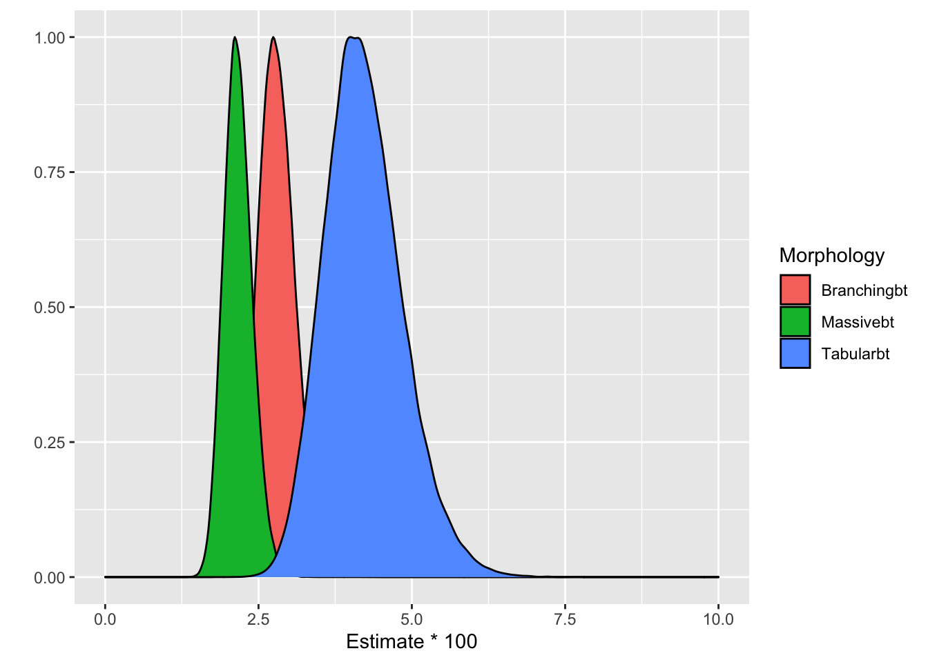

It is evident from the code that they plot the fixed effects estimates with their standard errors. This plot ignores the random effects and it only takes into consideration the variation of the fixed coefficients \(\beta_j\). To get an idea for the variability of the random effects I simulate them from the model and plot them. Points that are distinguishable from zero (i.e. the confidence band based on level does not cross the red line) are highlighted. We see substantial variation on the random effects estimates with many “outliers” with both high and low averages that need to be accounted for.

library(merTools)
sim_rfs_Normal.Disease <- REsim(Normal.Disease.Growth, n.sims = 200) 
plotREsim(sim_rfs_Normal.Disease)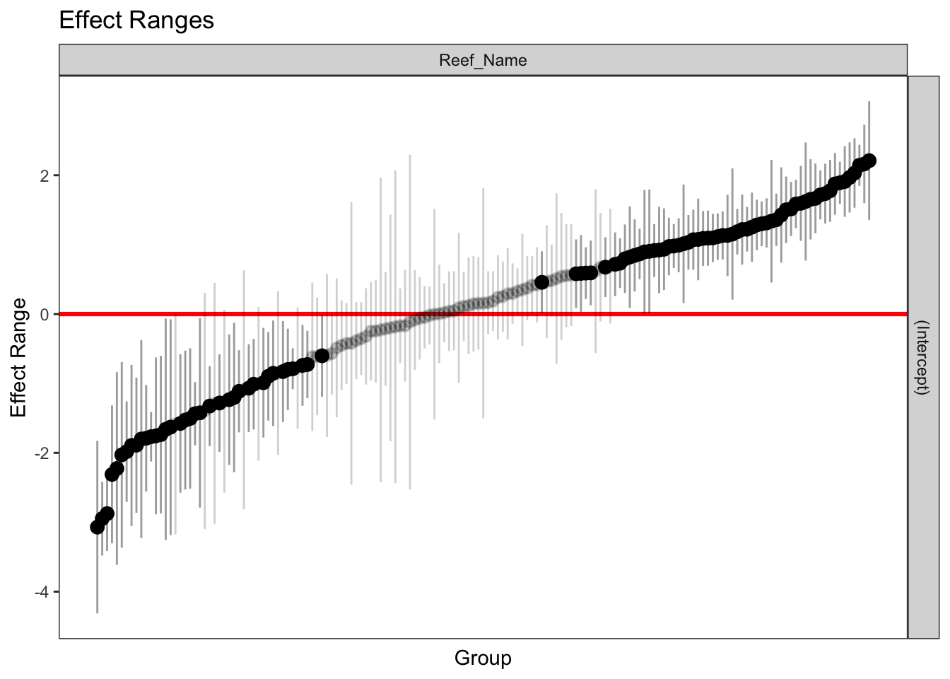

What the authors are effectively doing in Fig. 4(B) (see density plot above) is presenting the results for reefs with \(b_i = 0\) which corresponds to the red horizontal line. Let’s see how the density plot changes when we condition on more “extreme” reefs. I use the 0.1 and 0.9 quantiles.

quantile0.9 <- REquantile(Normal.Disease.Growth, quantile = 0.9, groupFctr = "Reef_Name")
#which(sim_rfs_Normal.Disease$groupID == quantile0.9)

quantile0.1 <- REquantile(Normal.Disease.Growth, quantile = 0.1, groupFctr = "Reef_Name")
#which(sim_rfs_Normal.Disease$groupID == quantile0.1)

NormalDisease.by.Growth_quantile0.9 = data.frame(
   Tabular = rnorm(100000, mean = -3.1332 + 1.495773, sd = .1549),
   Massive = rnorm(100000, mean = -3.8153 + 1.495773, sd = .1095),
   Branching = rnorm(100000, mean = -3.5534 + 1.495773, sd = .1103))
NormalDisease.by.Growth_quantile0.9$Tabularbt = plogis(NormalDisease.by.Growth_quantile0.9$Tabular)
NormalDisease.by.Growth_quantile0.9$Massivebt = plogis(NormalDisease.by.Growth_quantile0.9$Massive)
NormalDisease.by.Growth_quantile0.9$Branchingbt = plogis(NormalDisease.by.Growth_quantile0.9$Branching)
NormalDisease.by.Growth_quantile0.9 = gather(NormalDisease.by.Growth_quantile0.9, Growth, Estimate, Tabularbt:Branchingbt)
NormalDisease.by.Growth_quantile0.1 = data.frame(
   Tabular = rnorm(100000, mean = -3.1332 - 1.689569, sd = .1549),
   Massive = rnorm(100000, mean = -3.8153 - 1.689569, sd = .1095),
   Branching = rnorm(100000, mean = -3.5534 - 1.689569, sd = .1103))

NormalDisease.by.Growth_quantile0.1$Tabularbt = plogis(NormalDisease.by.Growth_quantile0.1$Tabular)
NormalDisease.by.Growth_quantile0.1$Massivebt = plogis(NormalDisease.by.Growth_quantile0.1$Massive)
NormalDisease.by.Growth_quantile0.1$Branchingbt = plogis(NormalDisease.by.Growth_quantile0.1$Branching)
NormalDisease.by.Growth_quantile0.1 = gather(NormalDisease.by.Growth_quantile0.1, Growth, Estimate, Tabularbt:Branchingbt)

NormalDisease.by.Growth$ID = "average"
NormalDisease.by.Growth_quantile0.1$ID = "0.1quantile"
NormalDisease.by.Growth_quantile0.9$ID = "0.9quantile"

overall <- rbind(NormalDisease.by.Growth, NormalDisease.by.Growth_quantile0.1, NormalDisease.by.Growth_quantile0.9)
ggplot(aes(x = Estimate*100, col = ID), data = overall) +
   geom_density(aes(y = ..scaled.., fill = Growth), alpha = 0.9, size = 1.3) +
   scale_fill_brewer(palette = "Spectral") + 
   #scale_fill_manual(values = c("#D55E00", "#009E73", "#0072B2")) + 
   scale_color_manual(values = c("#000000", "dodgerblue", "darkmagenta")) +
   scale_x_continuous(limits = c(0, 10)) + 
   ylab("") + 
   labs(col = "R effect", fill = "Morphology")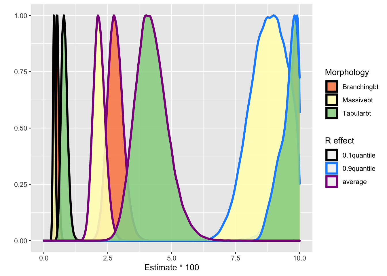

It is evident both the center and the variability of the distributions change depending whether we look an “average” coral reef (purple line), a reef towards the upper extreme (blue line) or the lower extreme (black line). So the conclusions should be something along the lines: the increase in disease likelihood with plastic debris depends also on inherit/unobserved characteristics of the reefs, captured by the random effects, in addition to their morphology.

Of course, what I have presented above is still conditional interpretation of the parameters. Ideally, we want the marginal population-average interpretation which is obtained from averaging over the random effects. This allows to take into account both the residual (observation-level) variance, the uncertainty in the variance parameters for the grouping factors added to the uncertainty in the fixed coefficients. See for example the predictInterval() function of the merTools package.

References

Lamb, JB, BL Willis, EA Fiorenza, CS Couch, R Howard, DN Rader, JD True, et al. 2018. “Data from: Plastic Waste Associated with Disease on Coral Reefs.” Science. Dryad Digital Repository. https://doi.org/10.5061/dryad.mp480.
Lamb, Joleah B, Bette L Willis, Evan A Fiorenza, Courtney S Couch, Robert Howard, Douglas N Rader, James D True, et al. 2018. “Plastic Waste Associated with Disease on Coral Reefs.” Science 359 (6374): 460–62.