Iridescence as camouflage - A comment on competing risks
Standard survival data measure the time span from some time origin until the occurrence of the event of interest. In the interpretation of results of survival analyses, competing risks can be an important problem. Competing risks occur when subjects can experience one or more events which ‘compete’ with the event of interest. In those cases, the competing risk hinders the observation of the event of interest or modifies the chance that this event occurs.
Here, I use the data from Kjernsmo et al. (2020) on biological iridescence to study the impact of competing risks on the final conclusions. First, I introduce the topic of iridescence and its intriguing biological significance (Background). Then, I outline the main idea behind competing risks (About competing risks) and present the two main types of hazard functions. I then re-analyse the data from Kjernsmo et al. (2020) (Results) and finish with a few concluding remarks.
Background
Biological iridescence (the vivid, shining colouring of many species) often serves to make individual animals more visible, and as a result, has been hypothesised to contribute to sexual selection. But the fact that it is found in non-reproductive stages makes the sexual selection hypothesis less likely. An alternative (and ) hypothesis is that can work as a form of protection, aiming “to conceal rather than reveal” .
Kjernsmo et al. (2020) provide evidence for this hypothesis by showing that iridescence provides a survival advantage making the prey less detectable, effectively acting as camouflage.
The authors use a coloured beetle species as a test case. The beetle’s wings sport a shiny, shifting and metallic green-blue appearance stemming from structural colour. They then use a series of elegantly simple experiments to test the camouflage hypothesis. First, they put together a collection of hundreds of beetle wing cases, including the iridescent and non-iridescent beetles in a variety of colours, and distributed them in a natural setting amid a variety of plant species. They found, surprisingly, that the iridescent specimens were more likely to survive predation by birds than the non-iridescent variety—even outperforming a leaf-green non-iridescent model that should have blended in with the background colours.
These conclusions are based on a mixed Cox model where the survival of the beetles was recorded at 2, 24, and 48 h. Predation by birds, which ate all or most of the metalwork, was scored as an event in the survival analysis. Predation by animals other than birds (non-birds), complete disappearance of a target, or survival to 48 h, were treated as censored values in the survival analysis1.
Effectively this analysis ignores the competing risks. A competing risk is an event whose occurrence precludes the occurrence of the primary event of interest. Being eaten by other animals precludes to be eaten by birds! Here, I re-analyse the data taking into account the competing risks.
About competing risks
Competing risks concern the situation where more than one cause of failure is possible. It refers to situations where an event has occurred, which prevents occurrence of the primary event of interest. For instance, in this study, predation by non-birds prevents the occurrence of the primary event of interest, i.e. predation by birds. A common assumption is that upon removal of one cause of failure, the risk of failure of the remaining causes is unchanged. That is, the competing risks are assumed independent. While this may be a reasonable assumption in some settings, independent competing risks may be relatively rare in biological applications.
When analyzing survival data in which competing risks are present, analysts frequently censor subjects when a competing event occurs (as done in this study). Thus, when the outcome is time to death attributable to birds, an analyst considers an insect as censored once it dies of non-bird causes (spiders etc). However, censoring insects at the time of death attributable to non-bird causes may be problematic (see Putter, Fiocco, and Geskus (2007) for a review). The next section introduces two ways competing risks can be taken into account.
The Hazard Function
A key concept in survival analysis is that of the hazard function. In the absence of competing risks, the hazard function is defined as
\[\lambda(t) = \lim_{\Delta t \to 0} \frac{Prob(t \leq T < t + \Delta t | T > t)}{\Delta t}\] where \(T\) denotes the time from baseline until the occurrence of the event of interest. The hazard function, which is a function of time, describes the instantaneous rate of occurrence of the event of interest in subjects who are still at risk of the event. In a setting in which the outcome is, say, all-cause mortality, the hazard function at a given point in time would describe the instantaneous rate of death in subjects who were alive at that point in time.
Competing risks implies that a subject can experience one of a set of different events - an insect can be eaten by a bird (event 1) or by a non-bird (event 2). In this case, 2 different types of hazard functions are of interest: the cause-specific hazard function and the subdistribution hazard function. The cause-specific hazard function is
\[\lambda^{CS}(t) = \lim_{\Delta t \to 0} \frac{Prob(t \leq T < t + \Delta t, \color{blue}{E = k} | T > t)}{\Delta t}\] The cause-specific hazard function denotes the instantaneous rate of occurrence of the \(k^{th}\) event (blue term) in subjects who are currently event free (i.e. in subjects who have not yet experienced any of the different types of events). If one were considering 2 types of events, death attributable to birds and death attributable to non-birds, then the cause-specific hazard of bird death denotes the instantaneous rate of bird death in insects which have not yet experienced either event (i.e., in insects that are still “alive”). The subdistribution hazard function is
\[\lambda^{SD}(t) = \lim_{\Delta t \to 0} \frac{Prob(t \leq T < t + \Delta t, \color{blue}{E = k} | T > t \color{blue}{\cup (T < t \cap E \neq k)})}{\Delta t}\] It denotes the instantaneous risk of failure from the \(k^{th}\) event in subjects who have not yet experienced an event of type \(k\) (blue term). Note that this risk set includes those who are currently event free as well as those who have previously experienced a competing event. This differs from the risk set for the cause-specific hazard function, which only includes those who are currently event free. Using the same example as above, the subdistribution hazard of predation by birds denotes the instantaneous rate of bird death in insects who are still “alive” (i.e. who have not yet experienced either event) or who have previously died of non-bird predation. There is a distinct cause-specific hazard function for each of the distinct types of events and a distinct subdistribution hazard function for each of the distinct types of events.
Note, the difference between the two hazard functions is in the risk set. As a result, for the cause-specific hazard, the risk set decreases at each time point at which there is a failure of another cause. For subdistribution hazard insects who fail from another cause remain in the risk set.
Here, I’m interested in modelling the effect of covariates on both hazards and see if that leads us to different conclusions.
Results
The data can be found here2. First, I transform the data for competing risks analysis. I use the following three event type indicators: 1 for bird death, 2 for non-bird death and 0 for censored observations.
# data transformation for competing risks
# data is the loaded data-frame
data_compete <- data %>%
    mutate(BirdPredated = case_when(
        (Notes == "SPIDER" | Notes == "ANTS" | Notes == "SLUG" | Notes == "WASP") ~ 2,
        TRUE ~ as.numeric(BirdPredated)))
I use the survival package to fit the two cause-specific models: cox1 for bird death and cox2 for non-bird death.
library(survival)

# Cause-specific hazard for bird death
cox1 <- coxph(Surv(Time, BirdPredated == 1) ~ Treatment, data = data_compete, x = TRUE)

# Cause-specific hazard for non-bird death
cox2 <- coxph(Surv(Time, BirdPredated == 2) ~ Treatment, data = data_compete, x = TRUE)
I then use the cmprsk package to fit the two subdistribution models: crr1 for bird death and crr2 for non-bird death.
library(cmprsk)
# necessary pre-processing
Treatment <- model.matrix(~ data_compete[, "Treatment"])[,-1]
cov_mat <- Treatment

# subdistribution hazard bird death
crr1 <- crr(data_compete$Time, fstatus = data_compete$BirdPredated, cov1 = cov_mat, failcode = 1)

# subdistribution hazard non-bird death
crr2 <- crr(data_compete$Time, fstatus = data_compete$BirdPredated, cov1 = cov_mat, failcode = 2)
I plot the hazard ratios (HR) with 95% confidence intervals for each treatment. We see that treatment affects the relative cause-specific hazard of bird death (red)3 but not of non-bird death (blue). Similarly, treatment has a significant effect on the relative incidence of bird death (green), but not of non-bird death (yellow). Together these indicate that, contrary to non-bird predators, birds are less sensitive to iridescent targets. Interestingly, though, treatment has a more accentuated effect on the cause-specific hazard (red) of bird death than the cumulative incidence (green) of bird death. Likely, the effects are qualitatively the same, which not be the case.
## Warning: Using `size` aesthetic for lines was deprecated in ggplot2 3.4.0.
## ℹ Please use `linewidth` instead.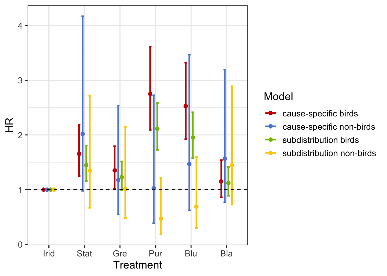
Which one to use?
This example demonstrates that the two approaches may yield different results. This can be explained by the different composition of the risk sets. In the cause-specific model for bird death, insects who died from a non-bird cause were censored and thus removed from the risk sets after their time of death, whereas they were kept in the risk sets after death in the subdistribution model.
As a result, the cause-specific hazard ratio (\(HR^{CS}\)) and the subdistribution HR (\(HR^{SD}\)) do not have the same interpretation. For example4, the \(HR^{CS}\) of 1.65 means that static rainbow insects (‘Stat’ in plot - red), had a hazard of dying 1.65 times higher than iridescent insects, among insects who were alive and did not die from non-bird predators. The \(HR^{SD}\) higher than one (\(HR^{SD}\) = 1.45) means that the cumulative incidence of death is higher in static rainbow insects (‘Stat’ in plot - green) when compared with iridescent ones. However, the numerical value of 1.45 is not straightforward to interpret since it reflects the mortality rate ratio among insects who are alive or have died from non-bird predators. So, the \(HR^{SD}\) is in fact a different quantity than an \(HR^{CS}\), representing a ratio in a non-existing population including those who experienced the competing event.
This quantity is mainly of interest for prediction. That is why the the subdistribution hazard ratio may be thought of as a measure of ‘prognostic association’, i.e. best suited to quantifying predictive relationships. This suggests that subdistribution hazards models should be used for developing clinical prediction models. Conversely, the cause-specific hazard ratio may be thought of as a measure of ‘aetiological association’, i.e. best suited to quantifying causal relationships and may be more appropriate for addressing questions of aetiology. (see Noordzij et al. (2013) for a comprehensive review and Feakins et al. (2018) for an application on cardiovascular and cancer mortality).
References
Predation by other animals included spiders, which sucked the fluids out and left a hollow exoskeleton, slugs, which left slime trails, and ants, which chopped off small pieces of the mealworm.↩︎
I use
Kjernsmo_et_al_Experiment1_data.txt↩︎These are almost identical results as in the original paper (Kjernsmo et al. (2020)), even though I don’t use any random effects.↩︎
These figures can be obtained from ‘summary(cox1)’ and ‘summary(crr1)’.↩︎